Bad theory drives out good: the only place where people can put their money is into someone else’s pocket. Quantitative Easing has contributed to fostering a pervasive belief in capital markets that the quantity of (central bank’s) money is all that matters, because - as the argument goes – “people have to put their money somewhere”, be it bonds, equities or alternative assets, such as cryptocurrencies. However, because it overlooks the critical role played by money velocity, this “liquidity paradigm” is both theoretically flawed and empirically contradicted.

A mere acquaintance with double-entry book-keeping indicates, indeed, that the only place where people can put their money is into someone else’s pocket. When Mr. X buys shares from Mrs. Y for cash, the former substitutes shares for cash in his assets, while the latter does the opposite in her assets. Money has not disappeared, it has just changed hands. In an extreme case, if market participants were to hoard the whole of their money balances, by design not a single transaction would take place and there would not be any asset price to observe. Therefore, it is not the quantity of money but its circulation that causes asset prices to rise or to fall. Yet, few people seem to consider the velocity of money in capital markets as a variable of interest.

Measurement issues are at least partly responsible for this neglect.
One cannot comprehensively observe how frequently money changes hands in all segments of capital markets. The nominal value of transactions executed in stock exchanges is usually known, but that is not the case for transactions executed in OTC markets or dark pools. As for the share of the money supply involved in financial transactions, it is anybody’s guess. For lack of a more comprehensive and granular measure, we shall define the financial velocity of money as the ratio of the equity turnover value to the broad money supply.

The unbearable fickleness of financial velocity. The neglect of the financial velocity of money is all the more puzzling as there is some evidence that central banks do not seem to control it. China is a case in point. Why investigate this issue in China? Because the observation conditions are probably better in China than elsewhere. Chinese equity markets and money supply have been and still are less open to foreign influence than their US counterparts. Chinese data on the nominal value of transactions are probably more comprehensive and reliable than the US ones.

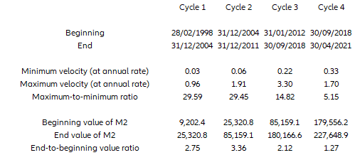
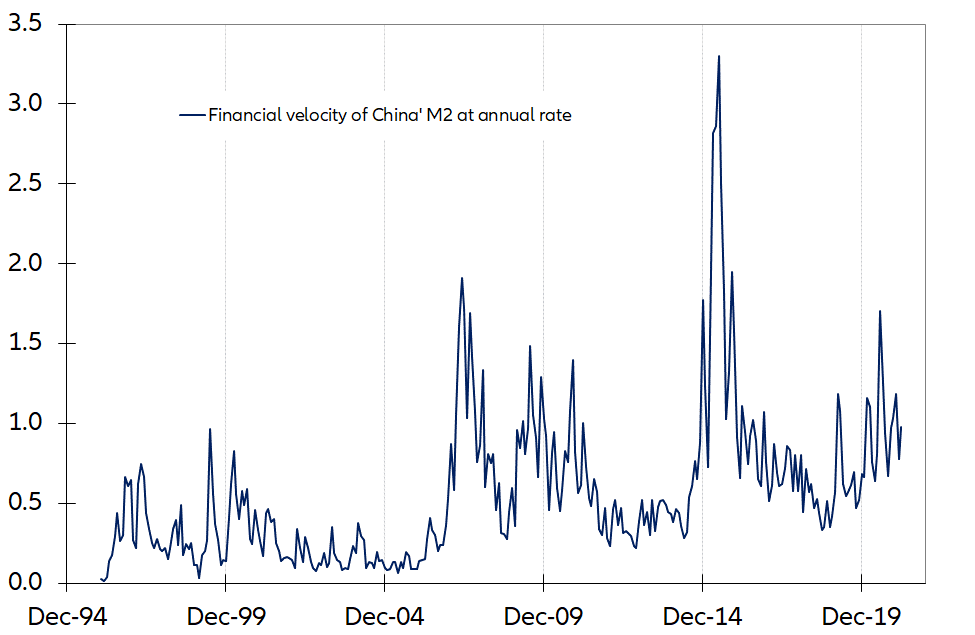
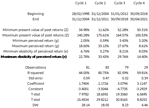
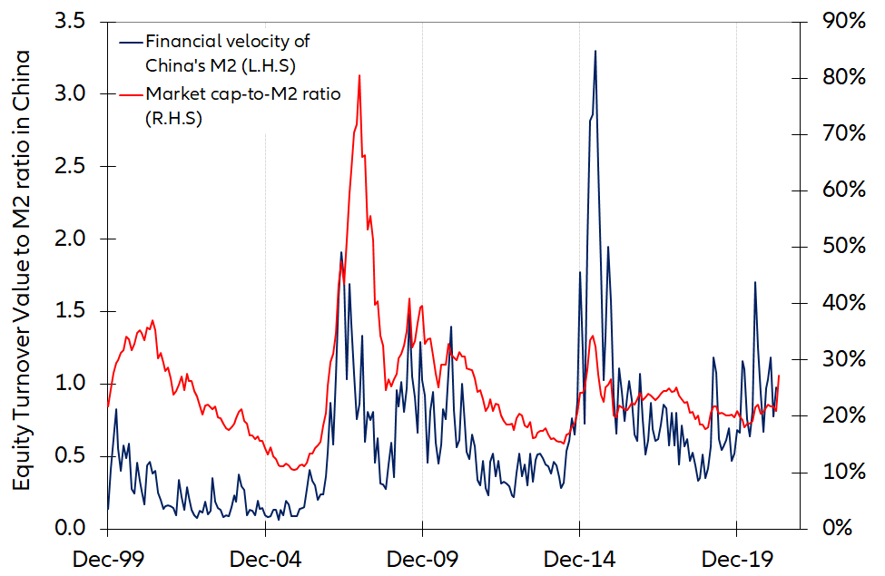
Our first key observation is that the financial velocity of money in China – defined as the ratio of equity turnover value-to-M2 – has been highly unstable1.  From the trough to the peak of the last three market cycles, the financial velocity of money has been multiplied by almost 30 and 15, respectively, as shown in Table 1 and Figure 1.

Table 1 – Extreme values of M2 and its financial velocity through cycles
Sources: Refinitiv/Allianz Research
Figure 1 – Ratio of equity turnover value-to-M2 in China
Sources: Refinitiv/Allianz Research
In contrast to its financial velocity, M2 has almost never kept growing from 1998 to date, but has only been multiplied by two to three between the end and the beginning of each of the three cycles. In other words, the financial velocity of M2 has been far more volatile than M2 itself.
           
By equity turnover value, we mean the sum of the Shanghai and Shenzhen stock exchange turnovers, expressed at an annual rate. As a result, financial velocity is also expressed at an annual rate.
The second key observation: none of the exogenous variables usually invoked to explain fluctuations in the velocity of money succeeds in explaining what we have witnessed in China: Neither (policy or market) interest rates, nor (narrow or broad) credit and money aggregates, nor the reserve requirement ratio, nor the exchange rate show any significant and stable correlation with financial velocity. Furthermore, over the same time, in the wake of a secular decline, the income velocity of M2 (the ratio of nominal GDP-to-M2), namely the velocity of money in the real economy, has halved.

Positive but non-linear feedback loops between past returns and financial velocity. Since we cannot explain the financial velocity of M2 with variables exogenous to the equity market, what about endogenous factors? Could there be, for example, a positive feedback loop between equity returns and financial velocity? As shown in Figure 2, we submit that this is indeed the case, subject to two assumptions.

Figure 2 – Ratio of equity turnover value-to-M2 and present value of past equity returns (Shenzen SE A shares index)
Sources: Refinitiv/Allianz Research
First, the sequence of past returns should be captured by what Maurice Allais would have called the “present value of the past returns” on the Shenzhen stock exchange A share price index. This present value of past returns Z is a weighted sum of past returns in which the recent returns are given more weight than the older ones and the weights decline exponentially, but not at a constant rate, this rate – or gain in the updating equation - being itself context-dependent, increasing – between 0 and 1 - when Z and/or the latest return increase, and conversely. In other words, the higher Z is, the greater its elasticity with respect to outcomes and therefore its potential instability. One can interpret this variable Z as measuring the market’s momentum. Its sibling, the perceived return z, is a weighted average of past returns, the weighting structure remaining the same; one can interpret it as an expected rate of return.

Second, the relationship between financial velocity and the present value of past returns should be assumed to be logistic, i.e. non-linear and bounded by two horizontal asymptotes, as shown in Figure 3, which describes this logistic relationship during the 2012-2018 cycle (cycle 3). Why make this logistic assumption? It is not only a matter of better closeness of fit. It is first and foremost because this logistic assumption eschews the two absurd conclusions to which the two other possible and more usual assumptions would lead. A linear relationship would not only open the possibility for financial velocity to be negative (!) when the present value of past returns is low, but it would also imply it could reach infinity at the other end of the spectrum, which is physically impossible. An exponential relationship would deal with the first absurdity, but not with the second one.

Figure 3 – The logistic relationship between the financial velocity of money and the present value of past equity returns in cycle 3
 Figure 3 – The logistic relationship between the financial velocity of money and the present value of past equity returns in cycle 3
Sources: Refinitiv/Allianz Research
Correlation, yes, but with causality. Table 2 provides the key stats of this logistic model for each of the three complete cycles we have witnessed since 1998. These three cycles share some common characteristics. They have had almost the same duration of about 80 months. The present value of past equity returns peaked at comparable levels, to which correspond perceived equity returns in the range of 20 to 30% a year. In cycles 2 and 3, the closeness of fit is remarkably high. The coefficients of the linear regression exhibit some instability, but they are always statistically significant.

More to the point, causality tests clearly show that the causality runs from the present value of past equity returns to the financial velocity of money. Not only is the sequence of past returns correlated with financial velocity but it is driving it. But how? A plausible transmission mechanism might work as follows: In the wake of a sequence of (mostly) positive and increasing large-cap equity returns, some market participants - let’s call them the early birds - become confident that the market is in a rising trend. They look at their portfolios and find that they hold too much cash and not enough large caps.

Table 2 – Key statistics
Sources: Refinitiv/Allianz Research
Out of a fear-of-missing-out (FOMO), they decide to dishoard a fraction of their precautionary money balances. Hitherto idle or dead, these balances become transaction balances on the hunt for large caps, bidding their prices up. Who are going to be the sellers?

As pointed out by John Kenneth Arrow, “models of the securities markets based on homogeneity of individuals would imply zero trade”, because all market participants would hold the same expectations and all strive to buy or sell at the same time2. So, the sellers of large caps in this first round must have different expectations. Some may not share the view that the market is in a rising trend: they look for fresh money with the intention to hoard it. Others, trying instead to be a few steps ahead, may expect this initial liquidity flow to trickle down to riskier assets, like small caps, junk bonds, you name it: they look for cash with the intention to employ it likewise.

In any case, since - as said above - the quantity of cash in the system remains the same, while equity prices are rising, the market capitalization-to-money ratio is rising3. This is why, as shown in Figure 4, China’s financial velocity of money and the market capitalization-to-money ratio tend to move in the same direction at the same time.

Figure 4 – Financial velocity of M2 and the market capitalization-to-money ratio
Sources: Refinitiv/Allianz Research

And, as equity prices have risen again, confidence now spreads to those market participants who had hitherto stayed on the sidelines.
As a result, some additional precautionary balances are dishoarded and put at work, which - round after round - reinforces the positive feedback loop between past equity returns and the financial velocity of money. At some point, some market participants - thinking that there is no alternative (TINA) to buying equities – will be doing so by borrowing money. As shown in Figure 5, the financial velocity of M2 and outstanding margin debt tend to move in the same direction at the same time.

Figure 5 – Financial velocity of M2 and margin debt

Figure 5 – Financial velocity of M2 and margin debt
Sources: Refinitiv/Allianz Research

There is no alternative, but there may be some limits. Theory and observation both suggest that there might be an upper limit to the appreciation of equity prices. The first limit is the equity market capitalization, which represents part of the nominal stock of productive capital. From the assumption that the marginal productivity of capital is declining, the theory of capital draws the conclusion that the capital-to-output ratio should be fairly constant through time. Notwithstanding the difficulty of measuring the stock of capital, this conclusion is broadly compatible with observed data. Hence, if the overall capital-to-output ratio is fairly constant, the components of the capital stock – including the part represented by equities – cannot have an unlimited headroom.

The second limit is the very dynamics of positive feedback loops. The driving force – the present value of past returns (or its sibling, the perceived equity return) – is akin to an ogre that can get stronger only if it is fed with ever-increasing returns. For example, as shown in Table 2, at the peak of cycle 2, the perceived equity return the reached the level of 33.1% a year (or 2.4% a month). For the perceived equity return to reach a higher level, the Shenzhen stock exchange A share price index had to deliver a monthly return higher than this 2.4% monthly equilibrium rate. However, then this hurdle rate would not only increase again, but also become more vulnerable as its elasticity to adverse outcomes would rise further. Herein probably lies the reason why markets sometimes give the impression of crumbling under their own weight without the help of any exogenous shock or trigger.

As shown in Figure 4, another reason probably lies in the fact that as the present value of past returns (and therefore the velocity of money) increases, the market portfolio becomes increasingly exposed to equities, thus reducing the gap between the desired and the effective portfolio structure and, therefore, the need for marginal portfolio adjustments. When almost everybody is already long equities, it is getting more and more difficult to draw in new buyers and to have more money change hands. This would explain why an upper horizontal asymptote ends up capping the financial velocity of money.

So much for Chinese data.

A flash back on Wall Street in the roaring twenties. Before discussing what policymakers and market participants should make of these observations, let us further observe that China is not the only place in the world where positive feedback loops are to be observed. The behavior of the financial velocity of money in the US during the roaring twenties illustrates how they have occurred in other places and times.  

The sum of the debits on deposit accounts in a given bank measures the money spent by its depositors during a given period. Hence, the sum of the bank debits in the banks of a major financial center can be taken as a proxy for the nominal value of financial transactions executed there.

A time series to be found in the NBER macro history database pertains to bank debits in New York City from 1918 to19414.  As shown in Figure 6, bank debits in New York City increased by an average 15.4% a year between the end of 1923 and September 1929. To be fair, bank debits outside NYC also increased, but at a third (5.2%) of the NYC rate5.

Figure 6 – NYC bank debits and the present value of past equity returns lagged one month from 1918 to 1933

Figure 6 – NYC bank debits and the present value of past equity returns lagged one month from 1918 to 1933
Sources: NBER macro history database /  Allianz Research
Almost two thirds of the total increase in NYC bank debits happened between December 1926 and September 1929, a period during which they grew at an average rate of 17.1% a year, while bank deposits grew by only 3.1% a year6. Hence, up to a quasi-constant divisor, NYC bank debits provide a proxy for the financial velocity of deposits.

As Wall Street crashed and the US economy entered into the Great Depression, bank debits contracted faster in New York (-32.5% a year on average from September 1929 to December 1932) than outside
(-20.8%), but also faster than deposits (-10.9%). Particularly noteworthy is the fact that the contraction in bank debits preceded the contraction of bank deposits: In other words, money velocity contracted before the money supply. This is not surprising. When the velocity of money falls, spending and income fall, too, and bad loans and in the end defaults rise.

Last but not least, as shown in Figure 7, despite being almost a century and 12,000 km apart, NYC bank deposits in the 1920s are in the same kind of logistic relationship to the present value of past returns as the financial velocity of M2 in contemporary China7.  

Figure 7 - NYC bank debits and the present value of past equity returns from 1918 to 1933
Sources: NBER macro history database / Allianz Research
When history meets experimental economics. In Figure 6, the present value of past returns is lagged by one month. Because of this lag, bank debits and the market seem to have peaked simultaneously. But in fact, while the market reached a record high in September 1929, bank debits peaked one month later. This belated spike in transactions probably means that, after a multi-year rally, one single month of negative return is not enough to dent the buy-the-dip (BTD) mentality. More than once, the early phase of a bear market has been interpreted as a “healthy correction”. Be that as it may, a closer look at Figure 6 shows that, leaving aside this isolated spike in October, bank debits actually peaked in January-March 1929, six to eight months before Black Thursday. That the value of transactions peaks before prices is a pattern also found in Vernon Smith’s laboratory experiments on asset markets8.  

To lean or not to lean against the wind. Whether and how central banks should pay attention to equity prices is a perennial debate. The case for neglecting equity prices rests on the premise that if markets are efficient, there is no reason to believe that central bankers could better discover the fair value of equities than private agents. There are enough unobservable variables (the equity risk premium, the long-term expected growth rate) and therefore degrees of freedom in a dividend discount model to make this conclusion hardly controversial.

But if equity markets are not always efficient, if – as suggested above - they happen to be prey to positive feedback loops where expectations and behavior depend on past outcomes, then the case for neglecting equity markets falls apart. Waiting for a positive feedback loop to crumble under its own weight, once it inevitably reaches its “natural” limits, is not an option, because such a policy would foster an accumulation of potentially bad debts. One can say, as Jay Powell did recently, that “asset prices are high” and “parts of the markets are a bit frothy”. But even if models – like the (in)famous Fed model - support such a statement, owing to model uncertainty, it sounds more like a value judgement than a mere observation of what market participants actually do rather than say.

Some of these behavioral variables - like the financial velocity of money, margin debt, the equity market capitalization-to-money ratio discussed above or the volume of margin deposits with clearing houses shown in Figure 8 - lie almost in plain sight9.  

Figure 8 – A proxy for margin deposits with US clearing houses
 Figure 8 – A proxy for margin deposits with US clearing houses
Sources: Refinitiv / Allianz Research
Shouldn’t such variables inform policymaking?  For example, coming back to China, the current and concomitant rise in the financial velocity of M2, in the market capitalization-to-M2 ratio and in margin debt – albeit less pronounced than in cycles 2 and 3 – should tell the central bank that the equity market does not need additional liquidity injections to say the least.

Isn’t it paradoxical that, despite having IT at our service, we are not currently collecting data – like bank debits – that were available a century ago? Why is it easier to monitor the nominal value of equity transactions in China than in the US or in Europe?

Even if moral hazard were nonexistent, monetary policy is admittedly ill-equipped to contain upward positive feedback loops: why should market participants care about a 50 bps hike of policy rates when, right or wrong, they “expect” equity returns in the range of 20% to 30% a year? But monetary policy can easily exacerbate upward positive feedback loops through forward guidance or by increasing the supply of money when the financial velocity of money is already on the rise. Clearly prudential regulation has a major role to play. When and how are questions that are not within the scope of the present work.

Liquidity is one of the most dangerous words in finance. What does our investigation mean for practitioners? It means that the word “liquidity” is one of the most dangerous words in finance because it designates both a stock and a flow, the quantity of money and its velocity. As we have seen, the velocity of money in financial markets is, by and large, more volatile than the quantity of money. But it is not fluctuating randomly. The financial velocity of money is very much pro-cyclical. Admittedly, when market participants start to fret about a market capitalization-to-money ratio they deem too high, an increase in the money supply above its desired level can substitute for a fall in prices and restore some balance.

However, such an intervention will follow rather than precede a fall in the velocity of money, and – to be successful – it must be timely, adequately calibrated, credibly communicated and not allocated to deleveraging. In QE we may trust, but not without a few caveats. With many market participants seemingly overlooking the fact that the velocity of money (the flow of “liquidity”) is not only pro-cyclical but also far more unstable, especially in financial markets, than its quantity (the stock of “liquidity” generated by QE), the potential for endogenous financial instability is unusually high.