Executive summary

  • Market-based long-term inflation expectations – as revealed by index-linked bonds or inflation swaps – tend to concur. They are meaningful because capital markets participants are incentivized to price them as accurately as possible: more directly than other agents, they have skin in the game.
  • Market-based inflation expectations have two components: on the one hand, a long-term, adaptive (or backward looking) component, which is linked to the perceived (or cyclically-adjusted) rate of inflation and, on the other hand, a short-term, rational (or forward-looking) component, which can be proxied mainly by the ISM employment index and secondarily by the oil price. As the adaptive component exhibits some inertia, it holds both the rational component and inflation expectations on the leash.
  • At their current level, which is close to fair value, inflation expectations no longer present investors with any kind of safe bet. For this to happen again, transient cyclical forces must first pull them away from fair value.
  • As the cyclically-adjusted rate of inflation is currently rather inelastic, it would take quite a dramatic and persistent inflation surprise to have a material, structural impact on market-based inflation expectations. Given the current low elasticity of the anchor of market-based inflation expectations and the stability of core inflation expectations, any tightening of monetary policy is likely to be cautious.

Inflation expectations matter

Inflation matters for at least two reasons, first, because it forces transfers of wealth between debtors and creditors, second, because - by blurring the information contained in relative prices -  it makes economic calculus more difficult. But, inflation expectations matter even more, because they are liable to reinforce any inflationary process by altering people’s behavior.

Extreme conditions, be it acute deflation, like in the US during the Great Depression, or hyperinflation, like in Germany in the early 1920’s, or stagflation, like in the 1970’s, provide us with a magnifying glass: they highlight how expectations of rising or falling prices can amplify inflationary or deflationary dynamics through positive feedback loops.

This explains why inflation expectations nowadays play such a central role in the conduct and explanation of monetary policy. Knowing that Central Banks pay attention to inflation expectations, financial markets also do so.

But this is easier said than done, for inflation expectations are not directly or easily observable. Nor is it straightforward to understand what drives them. The purpose of the present investigation is to shed some light on these two issues.

Inflation expectations are best revealed by those who have skin in the game

Initially and for a long time, surveys have been the only way to gauge people’s inflation expectations. But the answer given to a survey very much depends on how questions are asked. Furthermore, people don’t necessary put their money where their mouth is.

These are two strong reasons to turn to financial markets, more precisely to inflation-linked bonds, to elicit inflation expectations. Such bonds, also known as linkers, are indexed to inflation so that the principal and interest payments rise and fall with the rate of inflation. In them are embedded implicit market-based inflation expectations, which one can derive from an arbitrage relationship between bonds bearing a fixed nominal rate of interest and inflation-linked bonds. The breakeven inflation rate is indeed the difference between the yield of a nominal bond and an inflation-linked bond of the same maturity. For example, the nominal yield on a 10-year UST is (at the time of writing, i.e. January, 31st, 2020) 1.52%, while the indexed or real yield on a 10-year UST linker is only -0.14%. For the linker to return as much as the nominal bond, inflation must run on average at at least 1.66%a year (=1.52-(-0.14)) over the next ten years. The breakeven inflation rates are very much the same across maturities.

So far, so good. But what if nominal yields or real yields happen to be distorted by some structural factors? Couldn’t these breakeven inflation rates be biased in one direction or the other?

Market-based inflation expectations concur (more or less)…

A worrywart might argue that quantitative easing (QE, i.e. the purchase of nominal bonds by Central Banks) artificially depresses nominal yields. Everything else being equal, quantitative easing would then lower market-based inflation expectations. In plain English, Central Banks would be using a biased weighing scale, could even be tempted to stack the deck, market-based inflation expectations would systematically underestimate inflation expectations. Another worrywart might also argue that, the linkers market still being a rather small one, there is a scarcity or liquidity premium in the linkers’ real yield that artificially depresses it. At least partially, this scarcity would offset the impact of QE.

That the linkers’ breakeven inflation rates should be taken with a pinch of salt is suggested by another, newer category of financial instruments, namely inflation-linked swaps. In an inflation swap, one party pays a fixed rate cash flow on a notional principal amount (the swap rate),  while the other party pays a floating rate linked to an inflation index. The latter bets that future inflation will remain below the swap rate. Like in any other swap transaction, an inflation-linked swap involves a limited use of liquidity. The pricing of an inflation-linked swap is therefore less liable to be distorted by QE than that of a linker.  Across maturities, the inflation-linked swap rates are currently 20 bips higher than the breakeven inflation rates.

Most importantly, breakeven inflation rates and inflation swap rates have been strongly correlated ever since these two types of instruments have coexisted: in other words, up to an almost constant spread of 30 +/-7 bips, they have been telling the same story in terms of market-based inflation expectations; while their levels have always slightly differed, they have always moved in the same direction and with the same intensity.

… but err more often than not

What does this mean? It means that the relevant question should not be the quest for a perfect measurement of inflation expectations, for it is probably impossible to design. The relevant question is rather to understand what drives the long-term as well as the short-term movements in the somewhat noisy measurements of inflation expectations that financial markets provide.

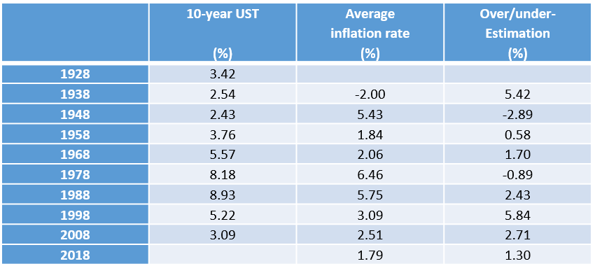
Let us start with the long-term movements. In theory, the buyer of a long-term bond, say a 10-year bond, should have an informed idea of the average inflation rate over the next 10 years. Hence, at the very least, the nominal yield on the 10-year UST should at any time be reasonably higher than the average inflation rate observed during the 10 subsequent years. As shown in Table 1, this has rarely been the case during the last nine decades. To take two extreme and opposite examples, in December 1938, the yield on 10-year UST was 2.54%, while the average inflation rate between 1938 and 1948 turned out to be 5.43%, leaving investors with an ex post negative inflation surprise of -2.89% a year. Conversely, in December 1988, the yield on 10-year UST was 8.93%, but the average inflation rate between 1988 and 1998 was only 3.09%, leaving investors with a positive inflation surprise of 5.84% a year.

In other words, the historical record shows that bond markets have done a poor job at forecasting the long-term trend in inflation. This should not be surprising, because inflation is not a risk, not an unknown unknown; it rather is an uncertainty, for we don’t know what cannot happen five, ten, twenty years out.

Table 1

Table 1
Source: Allianz Research

The cyclically-adjusted rate of inflation keeps market-based inflation expectations on leash

In an uncertain world, in a world of unknown unknowns, as Frank Knight put it, “we judge the future by the past…prophecy seems to be a good deal like memory, on which it is based”. As a matter of fact, market-based inflation expectations are linked with averages of past inflation rates, in which the weight given to a data point declines exponentially with its distance in the past: in other words, recent observations matter more than older ones. Such a non-equally weighted moving average measures what people perceive to be a “normal” rate of inflation after smoothing out cyclical fluctuations: hence, we can call it the perceived rate of inflation or the cyclically-adjusted rate of inflation. Its value as of January, 31st 2020 is 2.31% a year in the US. Interestingly, this number is remarkably close to the average long-term inflation forecast currently made by supposedly very rational economic agents, namely, first, the members of the Federal Reserve Board’s Federal Open Market Committee (2%) and, second, the professional forecasters surveyed by the Federal Reserve Bank of Philadelphia (2.2%). If this almost perfect alignment proves something, it is not that these three numbers will be proven right, but rather that they may be arrived at through the same not-so-rational thought process.

Like any kind of historic average, this cyclically-adjusted rate of inflation varies over time in response to fresh observation: it will rise or fall depending on whether the inflation rate observed in February is higher or lower (at annual rate) than 2.31%,  and so on.

As shown in Figure 1, this perceived rate of inflation or cyclically-adjusted rate of inflation has pretty much kept the breakeven inflation rate on leash. According to our proprietary valuation model, the breakeven inflation rate is proportional to the cyclically-adjusted rate of inflation up to an average estimation error of 40 bips (see model 1 in Appendix II). Since 2003, both in- and out-of-sample, the breakeven inflation rate has spent most of the time within the 90 bips range (or 68% confidence interval) indicated by the model. Strictly speaking, the relationship displayed on Figure 1 does not allow to forecast breakeven inflation rates even one month ahead, but it provides two important pieces of information.

First, it maps the distribution of potential outcomes and tells us whether it is symmetric or asymmetric.

Second, it measures the impact of any given inflation scenario of the cyclically-adjusted rate of inflation.

At their current level, which is close to fair value, inflation expectations no longer present investors with any kind of safe bet.

As the deviations from the model’s estimates are normally distributed, Figure 1 is, at any time, akin to a probability table. To illustrate this point, let’s look at Table 2, which maps the situation in Q2 or Q3 of 2018, as markets were still very confident about the global growth outlook and had not started to worry about trade tensions. The inflation breakeven rate was then slightly above 2.10, while the model’s estimate was 1.65. Put differently, there were nearly 7 chances out of 8 to observe a breakeven inflation rate lower than 2.10%  (and conversely only 1 chance out of 8 to observe a higher breakeven inflation rate). A further rise in the breakeven inflation rate could not be ruled out, but it was rather unlikely and if it did happen it would be limited in both magnitude and duration: in other words, the safe bet was that market-based inflation expectations would fall back, the risky bet that they would keep on increasing. The current situation is much more balanced: the 10-year breakeven inflation rate is only 7 bips above the model’s estimate (1.67 vs 1.59%). The current level of market-based inflation expectations does not present investors with any kind of safe bet. While the anchor of market-based inflation expectations is unlikely to move much in the near future, it is also unlikely to act as a magnet: cyclical forces are likely to pull market-based inflation expectations away from fair value. Let us now elaborate on these two points.

Figure 1

Source: Allianz Research
Figure 2:
Inflation
Source: Allianz Research

As the cyclically-adjusted rate of inflation is currently rather inelastic, it would take quite a dramatic and persistent inflation surprise to have a material impact on market-based inflation expectations

Let us now introduce some dynamics in the static analysis we have just conducted. The current value of the cyclically-adjusted rate of inflation is 2.3062% a year (or 0.1922% per month). For this perceived rate of inflation to move up or down, the next monthly inflation rate needs to be higher or lower than 0.1923%. How large this move might be depends on two factors:

  • first, something very uncertain: the magnitude of the inflation surprise with respect to 0.1922%
  • second, something known, at least in a not too distant future: the context-dependent elasticity of the cyclically-adjusted rate of inflation.

The first factor is rather intuitive: everything else being equal, the greater the surprise relative to 0.1922%, the larger the adjustment. This logic is embedded in classic exponential moving averages. It is in the second factor that lies the originality of Allais’s transformation: the higher the cyclically-adjusted rate of inflation, the higher its elasticity with respect to surprises. One would indeed expect people to be more wary of inflation surprises when they perceive inflation to be elevated than when it is perceived to be well-behaved: hence, the elasticity of the cyclically-adjusted rate of inflation should vary between 0, in a deflationary environment, and 1 in situations of hyperinflation.

As people have experienced many years of rather low and falling inflation, Allais’s transformation has it that the elasticity of the cyclically adjusted-rate of inflation is currently low: 0.6061% per month (or 7.2726% a year). If for example, the next monthly inflation rate were 0.6923% (or 8.31% annualized), the inflation surprise would be 0.51% per month (=0.6923%-0.1922%) and the cyclically-adjusted rate of inflation would rise by 0.0030% (=0.50% x 0.6061%) to 0.1952% per month (or 2.3427% a year). And the elasticity would rise from 0. 6061% to 0.6111%.

As shown in Table 3, right or wrong, our inflation forecasts do not imply any major surprises relative to the current value of the cyclically-adjusted rate of inflation. As such, they do not imply any major change in the future value of the perceived rate of inflation. In other words, we are not expecting the anchor of market-based inflation expectations to change much over the next four years; the range within which they will move should basically be stable: 1.59 +/- 0.45.

Table 3: US inflation forecasts

Source: Allianz Research
Figure 2
Source: Allianz Research

This does not mean that breakeven inflation rates will not move at all. To a certain extent, they will also reflect cyclical developments. 

We have been taking comfort from the fact that market-based inflation expectations deviate from the model’s estimate within a well-defined and stable range of +/- 45 basis points. In all fairness, we should also note that these deviations tend to be persistent. In other words, if we can rely on any deviation to vanish in the fullness of time, we cannot bet on this reversion to “fair value” to happen quickly.

This would be an issue if these residuals did not exhibit any pattern. But that is not the case. The residuals were positive before the Great Financial Crisis (from 2004 to mid-2008), they were also positive during the ensuing recovery (from 2009 to 2014) and again after the election of President Trump. Conversely, the residuals were negative when the dotcom bubble was still deflating (in 2002-2033), as well as at the height of the Great Financial Crisis (in 2008-2009), and again in 2015-2016 when the ensuing recovery ran a little bit out of steam.

Hence the idea of testing whether the residuals of our model might be correlated with a measure of economic confidence, like the ISM index. The test is positive: the residuals of model 1 are reasonably correlated with the ISM index (R-sq=50.26%). Actually, it is with the employment component of the ISM index that the correlation is the highest (R-sq=54.53%). This makes sense: it is “rational” (at least according to textbooks) to expect some wage inflation when employment is rising (see Figure 2)

Inspired by this observation, a model that purports to explaining market-based inflation expectations not only with the perceived rate of inflation (as in model 1), but also with the ISM employment index cuts the unexplained by half, as its average residual is +/- 26 bips (against +/- 45 bips previously). The residuals are also much less auto-correlated.

Taking a step back, such a model may be said to combine long-term adaptive (or backward-looking) expectations (i.e. the perceived rate of inflation) with short-term rational (or forward-looking) expectations (the ISM employment index). To that extent, it is strikingly similar to another of our proprietary model which explains the yield on 10-year US Treasuries by combining long-term adaptive expectations with short-term rational expectations. Like in this other model, the contribution of the rational expectations component – the bread and butter of Wall Street’s pundits - is not the most important of the two. Like in this other model, adaptive expectations keep rational expectations on a leash. Another short-term driver of market-based inflation expectations is the oil price.

Fluctuations in the oil price also explain some of the short-term movements in market-based inflation expectations

An investigation into the relationship between the oil price and inflation expectations typically starts with a figure like Figure 3, which – subject to a judicious scaling of the two vertical axes - overlays the USD 10-year inflation swap rate almost perfectly with the oil price. Graphs that display two time series on two different vertical axes are easy to draw and require little explanation. This is why the Street is so keen on using them to support narratives. But, being quick and dirty, such graphs are known to be misleading and short on quantification. Why should an oil price of USD 51.56 correspond to an inflation swap rate of 1.83%? Why should a level correspond to a rate of change?

It would seem to be more logical to link the inflation swap rate with some rate of appreciation in the oil price. But which one? The year-on-year rate of change? The month-on-month rate of change? Some weighted combination of short-, mid- and long-term fluctuations?

A classic exponential average addresses such questions by giving past observations, be they daily, weekly, monthly … rates of change, a weight that decreases with their remoteness, so that the most recent observations weigh more than the older ones. Allais’s transformation enhances this weighting scheme by increasing the weight given to the most recent observations whenever the pace of change tends to accelerate.

To illustrate the path-dependence embedded in Allais’s transformation, Table 6 displays the oil price, its perceived rate of appreciation and the latter’s elasticity at selected dates. These dates correspond to local highs and lows of the oil price during the last decade.

Table 4

Inflation expectation
Source: Allianz Research

Better than the oil price itself, its perceived rate of appreciation explains the inflation swap rate: up to a constant, the latter is proportional to the former (see model 2 in Appendix I and Figure 4). The presence of this constant is most interesting for it indicates the level of the inflation swap rate (i.e. 1.98%) given a zero perceived rate of appreciation of the oil price. In other words, it indicates the level of core inflation expectations.

Recursive estimates of this constant show that it has been remarkably stable. This is a most important observation, for it shows that – notwithstanding large swings in the oil price – core inflation expectations have barely moved up during the latest cyclical upswing.

While all of the above observations pertain to market-based inflation expectations in the US, the situation is very much the same in the EMU. The key difference is that in the EMU core inflation expectations are lower than in the US: 1.14 versus 1.98%.

Given the current low elasticity of the anchor of market-based inflation expectations and the stability of core inflation expectations, any tightening of monetary policy is likely to be cautious

Let us summarize our key findings:

  • the anchor of market-based inflation expectations, the cyclically-adjusted rate of inflation, is currently inelastic and will remain so;
  • core inflation expectations are low and have been stable during the latest cyclical upswing, notwithstanding large swings in the oil price.

Central Banks do not seem to use the smoothing methodology advocated in the present investigation (Allais’ transformation). Yet, they very much seem to reach the same kind of conclusions. Looking at these, Central Bankers are most likely to ask where is the fire; they are more likely to decide to wait and see rather than to rush into monetary tightening.

Like it or not, market-based inflation expectations are in fact data dependent. Hence, by taking them into account, Central Banks run the risk of being somewhat backward-looking, if not behind the curve. A worrywart might well wish Central Banks to be wiser, but the purpose of Central Banks’ watching is not to formulate what they should do, it is merely to forecast what they are most likely to do.

Figure 4

Chart4
Source: Allianz Research
Eric Barthalon
Head of Capital Markets Research