Emerging market sovereigns: turbulent times ahead?

EXECUTIVE SUMMARY

• Financial tightening in advanced economies and slowing trade growth have created less favorable conditions for emerging market sovereigns, which have been amplified by the effects of the war in Ukraine on commodity prices. While the capital accounts of emerging market sovereigns is often crucially influenced by the US monetary stance, their current accounts are very much dependent on demand from China due to their upstream integration in global supply chains.
• A repeat of sovereign debt crises similar to the ones in the 1980s and 1990s appears unlikely. However, several (large) emerging market (EM) economies have become highly vulnerable to tighter financing conditions, including those in Emerging Europe ( Hungary, Romania and Turkey) and Africa (Egypt, Kenya and Tunisia), as well as in Latin America (Argentina and Chile), albeit to a lesser extent.
• Under baseline conditions, we expect a broad-based but contained spread. In local currency terms, divergences between countries are as heterogeneous as inflationary pressures. Local currency yields will remain elevated in 2022, with a gradual reversal in 2023 as headwinds start to abate. Should our adverse scenario materialize, we expect the escalation of the war in Ukraine to cause a global recession with significantly higher inflation. Such a scenario would translate into a deterioration of EM fundamentals and generalized capital outflows, leading to a significant widening of hard currency spreads and a strong increase in local currency yields.
  

Even before the invasion of Ukraine disrupted capital markets, emerging markets and developing economies (EMDEs) were already facing a reversal of fortunes via both the capital and current account channels.

Capital Account Channel: Tightening US Monetary Policy

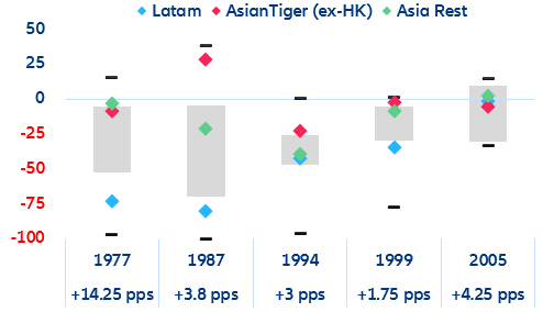
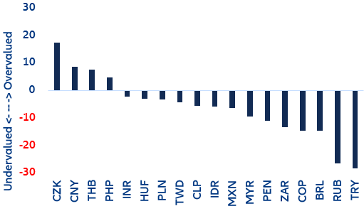
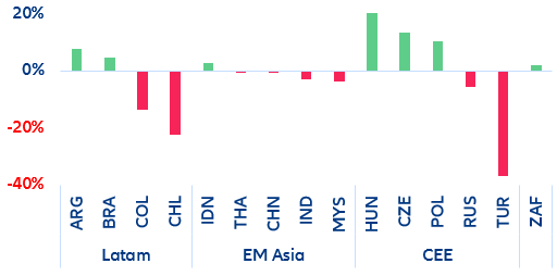
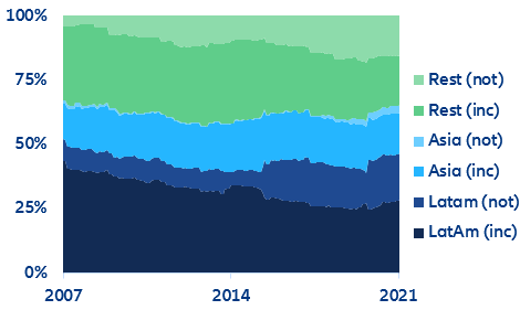
Financial conditions in advanced economies have significantly tightened since the beginning of the year; however, the US Federal Reserve’s shift to a hawkish monetary policy stance to combat surging inflation is also making investments in EMDEs less attractive in US dollar terms. As a result, countries will struggle to attract foreign capital as US real rates start rising, especially when their inflation is just as high (or even higher) than that of the US. Past evidence suggests that rising US rates tend to trigger significant FX pressures in EMDEs (Figure 1).
 
Figure 1: Impact of rising US interest rates on emerging market currencies (%)

Current Account Channel: Slowing Global Trade, Lower Demand from China and Eurozone, Rising Prices

While the capital account of EMDEs is determined by the US monetary stance, the current account is very much dependent on external demand from China and the Eurozone and, more broadly, global trade, with many EMDEs being deeply integrated upstream in global supply chains. However, the combined effects of the Ukraine war and renewed Covid-19 outbreaks in China have delayed the normalization of supply chains, weighing on global trade.  We expect global trade growth to slow to +4.0% in volume terms in 2022, while trade in value terms is bound to increase by +10.9%. So EMDEs’ current account balances are being affected by both volume and price effects through changes in external demand and the terms of trade.

EMDEs face a significant demand shock of more than 2% of GDP. We estimate that the Ukraine war could result in a loss of USD480bn in exports to Russia and the Eurozone this year, with countries in Emerging Europe most affected. Another source of vulnerability is Chinese demand, particularly from sectors that are affected by the national authorities’ zero-Covid approach and the crisis in the real estate sector. After accounting for revenues from purchases usually made directly abroad by Chinese residents, we find that the slowing Chinese economy could represent a drag of up to -0.6% of GDP for non-OECD countries; tailwinds from Chinese sectors that are likely to fare better in 2022 (infrastructure and manufacturing investment) are insufficient to make up for them (Figures 2 and 3).

Figure 2: Impact of slowing Chinese demand on selected groups of countries (%)

Figure 3: Trade dependence of selected advanced and emerging market economies in China

The impact of the terms of trade shock is sizeable but uneven (Figure 4):

• For net exporters: Large oil and gas exporters, such as Qatar, the UAE and Saudi Arabia, are likely to experience record increases in their trade-balance-to-GDP ratios due to higher prices and potential substitution effects away from Russia. Commodity exporters in other EMDE regions have also benefitted, especially some Latin American countries. They also offer high carry as central banks have raised interest rates significantly to battle inflation. The Brazilian real is the best-performing currency in the year (+18.4%), followed by the South African rand (+8.6%), the Colombian peso (+8%) and the Chilean peso (7.3%).
• For net importers: Countries such as Tunisia, Morocco and South Korea have been most affected by rising prices for fossil fuels and food. Net importers could potentially suffer from shortages and subsequent social discontent. The currencies countries such as India, Thailand and the Philippines have performed poorly in the year (-1.9%, -1.05% and -0.9%, respectively), alongside those countries of the CEE block (e.g. Polish zloty – 5.3%) notably affected by the ongoing geopolitical conflict.
  

Figure 4: FX performance in 2022 vs share of commodities in total exports

But how sustainable is the current commodity price push? While our FX valuation models point out that high-carry/commodity currencies are still cheap, hence supporting further appreciation for a while, there are several risks in the pipeline (Figure 5). On the domestic side, we observe increased political tensions in Latin America– e.g. upcoming presidential elections in Brazil and in Colombia, Constitutional changes in Chile – and rising risks of a new round of food shocks due to the rupture of fertilizer stocks as Russia is one of the main exporters of this product to several countries, including Brazil, Colombia and Chile which significantly increases risks of lower growth and puts additional pressure on inflation. On the external side, a conflict resolution in the background of tighter financial conditions in the US would certainly prompt investors to look back at the EMEs macroeconomic fundamentals, and hence growth outlook, fiscal consolidation and/ or reform agenda would be key. On this sense, countries such as Brazil have a much more fragile position.
 
Figure 5: Fair value of EMDE exchange rates (%)

Figure 6: Emerging markets import cover (months)

Figure 7: Terms of trade shock: impact of higher commodity prices on trade balances (% of GDP)

With this combination of factors affecting the capital and current accounts of EMDEs, the longer geopolitical tensions remain elevated and supply chains disrupted, the more challenging it will become to attract capital flows.

A repeat of the sovereign debt crises seen in the 1980s and 1990s appears unlikely, but some (large) EMDEs are at risk.

While most countries have gradually improved their external positions and built policy buffers over time, there are several (large) EMDEs that have become highly vulnerable to tighter financing conditions. Often, policy mistakes have aggravated the adverse impact of rising fiscal imbalances and external debt burdens. By assessing liquidity and cyclical risks, we find that the countries most at risk are in Emerging Europe ( Hungary, Romania and Turkey) and Africa (Egypt, Kenya and Tunisia), and to a lesser extent in Latin America (Argentina and Chile). Even without any further deterioration in geopolitical conditions, these countries are likely to struggle to rebalance their economies and avoid a continued deterioration of sovereign debt sustainability. A more detailed analysis on selected metrics can be found in Appendix 1.
 
Figure 8: EMDE vulnerability dashboard

Figure 9: Total return of EM sovereign bonds benchmark indices (indexed, 100 = end-Dec. 2004)

The currency duality of sovereign debt issued by EMDEs reflects the fact that many countries with less developed financial infrastructure seek long-term financing from abroad. After the tough decades of 1980 (“Latin America’s lost decade”) and 1990 (Asian crisis, currency crisis in Latin America, Russian default), the 2000s were a remarkable decade for EMDEs. The performance of both hard and local currency debt prior to the GFC – as well as for other assets, such equity – left was remarkable (Figure 9). However, everything changed in the decade of the 2010s. The taper tantrum, the drop in oil prices and in general the weaknesses of EM currencies created a divergence between the returns of both type of bonds, namely, an underperformance of bonds issued in local currency.

Figure 10: Net change in outstanding emerging market sovereign debt (2009-21) (USD billion)

Will current events change this divergence? It seems unlikely. So far, the main driver of changes would be the significant cross-financial sanctions between the US and Russia, in the form of FX reserves frozen by the former and fierce capital controls by the latter. This could mean a halt to globalization (both from the financial centers and from the finance-seekers), an increased distrust of the USD as the world reserve currency and further geopolitical pressures. Translated to the bond market, the first outcome to watch will be an even stronger division between hard currency issuance for foreign investors and local currency for local investors, but in principle this will not make local currency bonds more attractive. Appendix 2 provides further analysis on the differences between both types of issuances.

Most EMDEs have also tried to reduce their foreign-currency-denominated debt issuance (“original sin” ). However, some countries in Latin America and Emerging Europe still have a high share of hard currency debt (Figure 10 and Appendix 1).  

Figure 11: Change in the share of LC debt over total sovereign debt (2009 vs 2021)

What does this mean for hard currency spreads?

According to our calculations – and consistent with prior literature  – the main movements in the hard currency EM sovereign spreads are explained by changes in global financial conditions, while variables that refer to the fundamentals of the economy (GDP growth, inflation, FX reserves) are more relevant for explaining the levels, as well as the changes in times of financial calm. For simplicity, we consider corporate spreads in the main financial markets as proxy for global financial conditions, leave out some of the macroeconomic variables (global GDP growth or external debt) and calculate different coefficients depending on which is the hard currency (USD  and EUR ). To add a greater degree of heterogeneity, we include as an explanatory variable the oil price interacted with a dummy for oil-exporter countries. The parameters are estimated in a panel data framework, using first differences (yearly changes).

Before the Ukraine war, higher inflation had widened spreads, while recent rises in oil prices have helped improve debt sustainability of oil exporters. However, the contribution coming from US corporate spreads, which should have reduced the pressures, seems to be the element that has not transmitted as expected (although it is usually deemed as a good indicator of global financial conditions, there may be tensions that are not fully reflected via this channel). Going forward, we expect tighter global financial conditions to cause a broad-based but contained spread widening, also supported by inflationary pressures. In the event of a continuous deterioration of the Ukraine situation and a global recession, we would expect a significant widening of hard currency spreads.

Figure 12: Decomposition of the aggregate spread change of USD-denominated EM sovereign bonds

Figure 13. Relative face value of the region-level Bank of America (BofA) emerging market sovereign bond indices

Table 1: Calculated country weights in synthetic emerging market debt indices based on sub-samples of main emerging market sovereigns

Due to the complexity and number of countries, EM debt indicators are usually represented at an index level. However, due to our focus on major EM economies, we compose the index forecast from our individual country forecasts with different weights – and omit countries than are present in the official aggregates. In Figure 13, we show the relative face value of outstanding USD-denominated bonds included in country-level BofA of Latin America, Asia and rest and how much of the weights are covered by our reduced sample (the main regions not included are Central America and the Middle East). Table 1 shows the calculated weights: greater weights to Latin America, Turkey and two Asian countries, Indonesia and the Philippines. With the realized country-level spreads the weights are not substantially different, but with the estimated values we obtain a larger divergence. This difference can be explained by the different fit of the models for each country (e.g. the high share of Mexico and the low weight of South Africa).

How will local currency yields evolve?

According to our analysis, the main movements in local currency yields can be explained in the FX deterioration implied in the forwards markets. This, in turn, considers the reference interest rate differential and is consistent with the above-mentioned differences between local and hard currency spreads. The additional variables are inflation, real GDP growth and a global financial conditions factor. Both inflation and real GDP growth enter as exponential weighted averages trying to smooth the series to extract the long-term trend. Unlike in the hard currency spectrum, this variable has less relevance to explain movements.

The framework is again a panel data setting, with differentiated coefficients for Central Europe and other regions. The sample of countries is slightly different than in the hard currency universe, with more weight to Asian countries and less to Latin America. We again have 14 countries: Brazil, Mexico, Colombia (Americas); China, the Philippines, Indonesia, India, Thailand (EM Asia); Turkey, South Africa and Russia, Poland, Czechia and Hungary (Central Europe).
 
Figure 14: Decomposition of annual change in 5Y sovereign yields in Latin America

Inflation and higher policy rates were the drivers of big movements during 2021. In our baseline scenario we expect this trend to slow during this year, followed by a gradual reversal in 2023 as headwinds start to abate. Like the hard currency environment, in our adverse scenario we would see a much steeper increase in yields as fundamentals deteriorate and capital flees to safer assets (Figure 14).

Table 2: Calculated weight of EM index based on sub-sample of main EMs.

Both inflation and real GDP growth enter as exponential weighted averages trying to smooth the series to extract the long-term trend. Like the case of hard currency, the global indices include a wider scope of countries than we do as our focus is only on the main large EMs. As a result, we develop a similar analysis as the performed for hard currency spreads to try to build the benchmark indexes on smaller sample by calculating the country weights. Table 2 shows the obtained weights from both the country yields, the model-estimated country yields, and the real weights from reference benchmarks. These benchmarks usually try to diversify the weights as, if guided by amount outstanding, China would overwhelmingly dominate the movements. As in the case of hard currency, when using the model-estimated values, Mexico is overweighted while the contribution of both Thailand and the Czech Republic converges to zero.